Serial interface of DSO 068 oscilloscope
It’s time to describe how to use the serial interface of the DIY DSO 068 oscilloscope which I built back then. I used it extensively in Measuring Floppy Drive rotation speed - Part 4 and described the usage there. But it deserves a post on its own.
The oscilloscope
The DSO 068 is a simple oscilloscope with one channel capable of the easy things like trigger based capture of signals. It’s not too fast, but it’s still a “practical tool for everyday use”, to quote the elector website JYE Tech DSO068 Oscilloscope DIY Kit), where you can buy this DIY kit.
Here are the specs according to the data sheet:
- Max ETS (equivalent-time sampling) sampling rate: 20 MSa/s
- Max realtime sample rate: 2 MSa/s
- Analog bandwidth: 0-3MHz
- Sensitivity range: 10mV/div - 5V/div
- Max input voltage: 50Vpk (1X probe), 400Vpk (10X probe)
- Input impedance: 1MOhm / 20pF
- Resolution: 8 bits
- Record length: 256, 512, 1024 points (variable)
- Timebase range: 10min/div - 0.5µs/div
- Trigger modes: Auto, Normal, Single
- Trigger position range: 0% - 100%
- Frequency meter range: 5 MHz
- Frequency meter sensitivity: 0.2Vpp @ 5MHz
- Power supply: 3.7V Li-ion battery / USB
- Current consumption: ~300mA (with LCD backlight ON)
- Dimension: 140x70x30mm
- Weight: ~0.18kg (without battery and probe)
Besides being a “normal” oscilloscope, it has also a frequency meter built in and a FFT mode.
Send screen
It can be connected via USB to charge the battery or to have power at all. But it has also a serial
interface chip built-in, that means, you’ll see another serial port. For me the command lsusb -d 10c4:
displays this:
Bus 001 Device 012: ID 10c4:ea60 Silicon Labs CP210x UART Bridge
Through this serial port, the data that the oscilloscope captured, can be transferred to your computer for further analysis or create nice pictures.
This port runs with the usual settings 115200@8-N-1 (115200 baud, 8 data bits, no parity bit, 1 stop bit).
The data transfer between your computer (the “host”) and the dso happens with the help of the
x-modem protocol.
To use that under a Debian linux system, you’ll need to install the package lrzsz.
This contains the command line tool rx. With that, you can transfer the current screen of the DSO as a bitmap
to the host and also the current recorded data as a csv (comma separated values) file.
To transfer the screen, first plug in the USB cable. Then configure the correct speed for the serial port, e.g.
stty -F /dev/ttyUSB0 115200 (the device might vary). Then select in the DSO in the menu the option “send screen”.
After that, you can start the receiver via rx screen.bmp < /dev/ttyUSB0 > /dev/ttyUSB0.
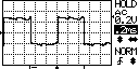
And the transfer begins. Note that the format is “BMP”. The order of the commands is important: First start the
transfer in the DSO. It will then wait for the receiver. Then start the receiver.
The result might look like this:
Send Wave data
The same way is possible for the data: menu option “send wave data” and
rx wavedata.csv < /dev/ttyUSB0 > /dev/ttyUSB0.
The format of the file is described in Capture Uploading and Waveform File Format. All these documentations for the DSO 068 can be found on the main page DSO 068 Oscilloscope DIY Kit.
Here I’m using the test signal at 5V and the 10X probe. On the screen you see roughly 2.5 divisions for the voltage level at 0.2V/div results in 0.5V and with the 10X probe it’s the expected 5V.
The CSV file looks like this:
JYDZ,Waveform,,,DSO068,JYE Tech Ltd.,WWW.JYETECH.COM
14,10,10
ChnNum,RecLen,ChnCfg,SampleRate,Resolution,Timebase,HPos,TrigMode,TrigSlope,TrigLvl,TrigSrc,TrigPos,TrigSen,TBcopy
00001,01024,,50000,00008,00023,00054,00001,00001,00143,,00010,,00023
00009
00001
00001
00001
2000
00009
00129


--------------------------------------------------------------------------------------------
00117
00117
00117
00117
00140
...
00141
00141
00115
00118
00118
00118
It starts with a header spanning multiple lines. There the settings are repeated:
- line 1: format is “Waveform”. This line could contain a date/time, if the device would know the actual time.
- line 2: contains three numbers:
- 14 is the number of fields in the next lines 3 and 4. Let’s count… field names are 14, values as well. That’s correct.
- 10 is the “vertical display resolution”. I guess, that’s something that can’t be configured and is always 10.
- 10 is the “horizontal display resolution”. Same.
- line 3: the fields names
- line 4: the values for the fields
- ChnNum = channel number. It’s always 1, as we have only one channel here.
- RecLen = record length. That can actually be configured and can be 256, 512, or 1024. In this example, it’s 1024.
- ChnCfg = channel configuration. Here we have no value.
- SampleRate = sample rate in Samples/second. 50,000 Samples/second. That’s important for how to interpret the samples starting at line 17.
- Resolution = Vertical capture resolution in bits. Here we have 8 bits resolution. That’s what this DSO is capable of.
- Timebase = this corresponds to the sec/div setting. 23?
- HPos = Horizontal position. I guess, that’s that the screen position.
- TrigMode = Trigger mode. 0 = auto, 1 = normal, 2 = single
- TrigSlope = Trigger slope. 0 = falling edge, 1 = raising edge
- TrigLvl = Trigger level. I have set it to 143. This needs to be interpreted in comparison with the reference below.
- TrigSrc = Trigger source. Not used.
- TrigPos = Trigger position. This can be configured and for me it’s 10%.
- TrigSen = Trigger sensitivity. Not used.
- TBcopy = Timebase. Same as the timebase field earlier in this line.
- line 5: vertical sensitivity. This is 9 for me. I guess, that’s the current setting for X5/X2/X1 and 1V/0.1V/10mV. That means: 9 = 0.2V, 7 = 1V, 6 = 2V, 5 = 5V, 10 = 0.1V, 13 = 10mV, 12 = 20mV, 8 = 0.5V, 11 = 50mV
- line 6: Couple. 2 = GND, 1 = AC, 0 = DC
- line 7: Vertical position.
- line 8: Vertical position offset.
- line 9: Sensitivity in unit of 0.1mV (absolute value). This is for me 2000. Since I have the setting “0.2V”, this matches: 2000 * 0.1mV = 200mV = 0.2V. So, no need to decode the vertical sensitivity setting.
- line 10: Vertical sensitivity - same as line 5.
- line 11: Reference. That’s the value corresponding to the 0V level. This is needed in order to interpret any value, like trigger level. The reference is for me 129. The trigger level was 143 - difference is 14. 14 units of 0.2V is 2.8V. So, my trigger level is at 2.8V.
After a couple of empty lines and a separator line, the actual data begins at line 17. Each line represents one sample. I’ve only kept in the sample above some values, e.g. in starts with “117”. This is using the reference of 129: 117-129=-12. -12 * 0.2V = -2.4V. A couple of samples later the value is at 141: 141-129=12. 12*0.2V=+2.4V. In total, we span roughly 4.8V, almost 5V, which is the test signal.
As each line represents a sample as a known sample rate, we can also figure out, how long e.g. the signal is at 2.4V: This is exactly 25 lines, if I counted correctly. If we assume, that the signal is periodic, this is only half the period. The whole period would be 50 lines. At 50,000 Samples/second, this means, it took 50/50,000 seconds = 1/1000 seconds. Which corresponds to 1000Hz, which is the test signal I used.
The whole captured CSV file is here: sample-dso-wavdata.csv.
Plotting
We could now use a spreadsheet program to draw a simple diagram out of the data. But there is also GNU plot. This can draw nice plots, if you know how.
There are some details to consider, like how to load the csv file, skip the 16 header lines at the beginning and scale the y axis, so that we can read the real voltage values. Most of this is described in the gnuplot manual and on stackoverflow, e.g. scale measurement data.
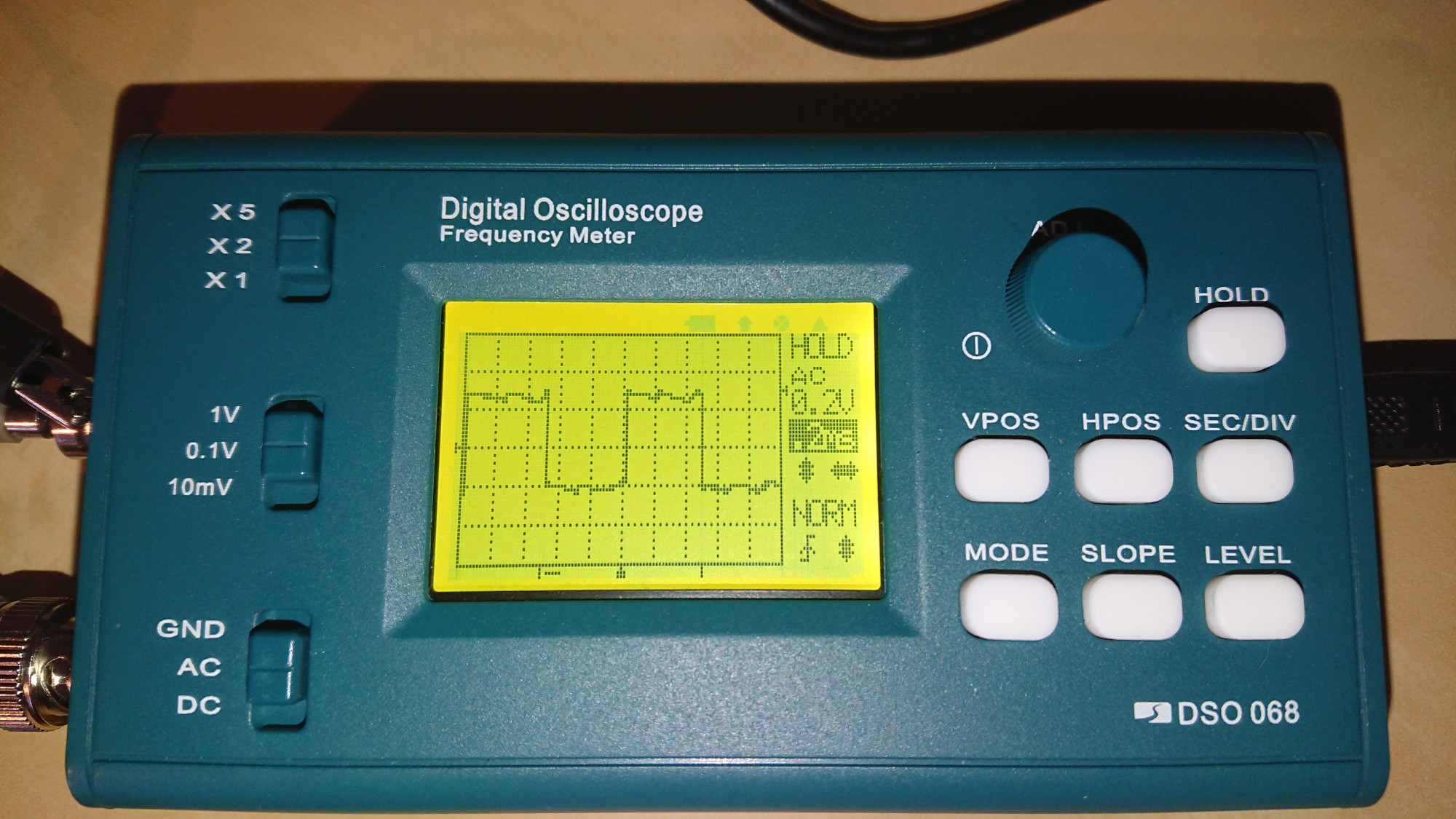
I came up with this script for gnuplot:
set terminal png size 800,400
set output 'sample-dso-wavdata.png'
set autoscale
set label " 2.4V" at 210,2.7
set label "-2.4V" at 235,-2.7
set title "test signal 1000Hz"
set ylabel "V"
set xlabel "samples @ 50,000Hz"
plot 'sample-dso-wavdata.csv' skip 16 using (($1-129)*0.2) with lines notitle
jyeLab
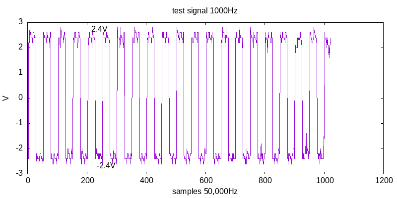
There is also jyeLab, a PC oscilloscope program. It supports “Realtime waveform display/capture”. However, this is a Windows-only program. The latest version 0.70 is from 2014, but it still runs on Windows 10. My virtual machine setup seems to be too slow to have a continuous data stream, but single shot mode works:
It also uses the UART USB connection. It would be an interesting project to reimplement this software to be available for linux as well. The protocol is documented at Data Interface.
Comments
No comments yet.Leave a comment
Your email address will not be published. Required fields are marked *. All comments are held for moderation to avoid spam and abuse.